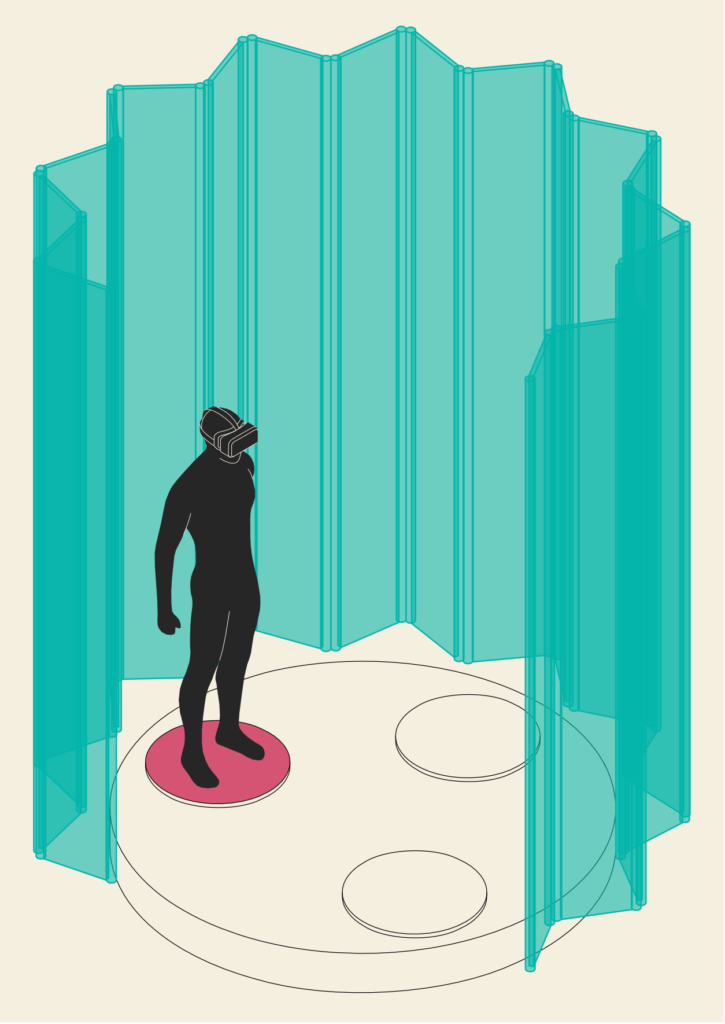
In this second experiment, we have chosen to create a moving surface that could help us to focus on the open/closed relationship between interior space and the surrounding environment. The different configurations that are generated have an effect on the user’s feelings. The configurations go from the maximum degree of privacy (shelter, protection) to a total mix between inside and outside (visibility, interrelation).
The proposed geometries are always connected to our Piattaforma Zero and together they form a new dynamic space system – Minimum Viable Space – that enriches our test laboratory to be explored in virtual reality.
Below is an in-depth analysis of the work process we used to generate the Folding Wall geometry with the help of Grasshopper, along with the relative tutorial to redo the experiment.
This geometry is composed of a set of panels connected by cylindrical hinges. Each panel rotates around its hinge causing the next panel to move. This type of relationship between the panels leads to a complex geometry capable of unfolding, thus changing its shape, from a closed to an open configuration. When the angle is set to 10°, the geometry contracts accordingly to the physics of the objects; when the angle is set to 90°, the geometry unfolds completely and traces the shape of a closed polygon.
Within our virtual environment Piattaforma Zero, we can select the desired surface and then, interacting with a slider, test all the possibilities given by the proposed movement. In the various structures of the experience, we can observe how the lights and shadows change inside the space and how the visual relationship between the user and the surrounding landscape is modified.
Let’s build it!
The geometry of the folding wall is developed within Grasshopper as follows:
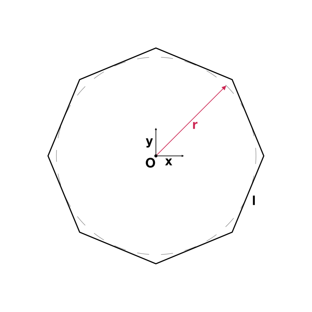
- Construction of the base polygon with a variable number of segments (n) and circumscribed to a circle having a variable radius called r. Depending on the combination of r and n, each segment of the polygon has a certain length l (Fig.1).
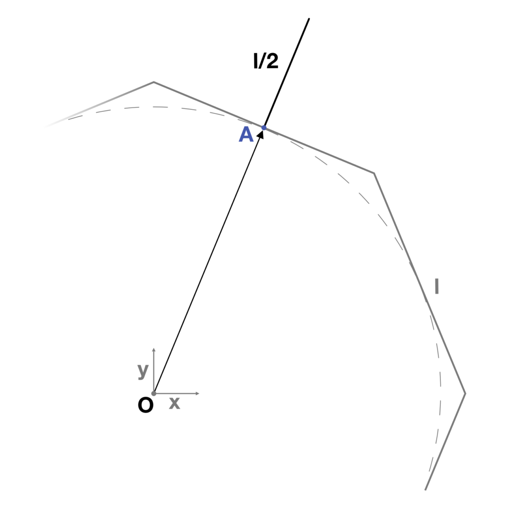
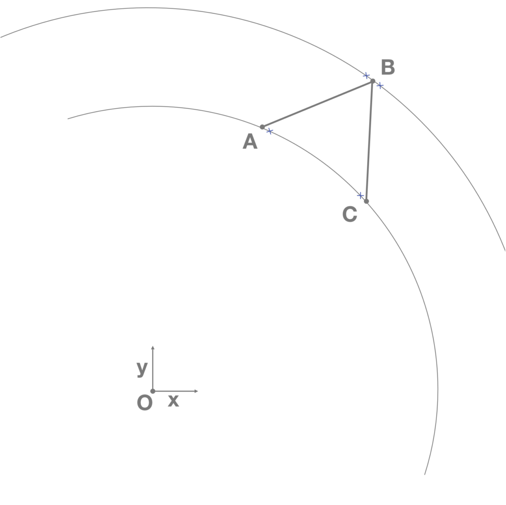
- Detection of the midpoint A on one segment of the base polygon. From A a straight line is constructed having the same direction of the vector between the origin of the base polygon and the point A and having a length equal to l/2 (Fig.2).
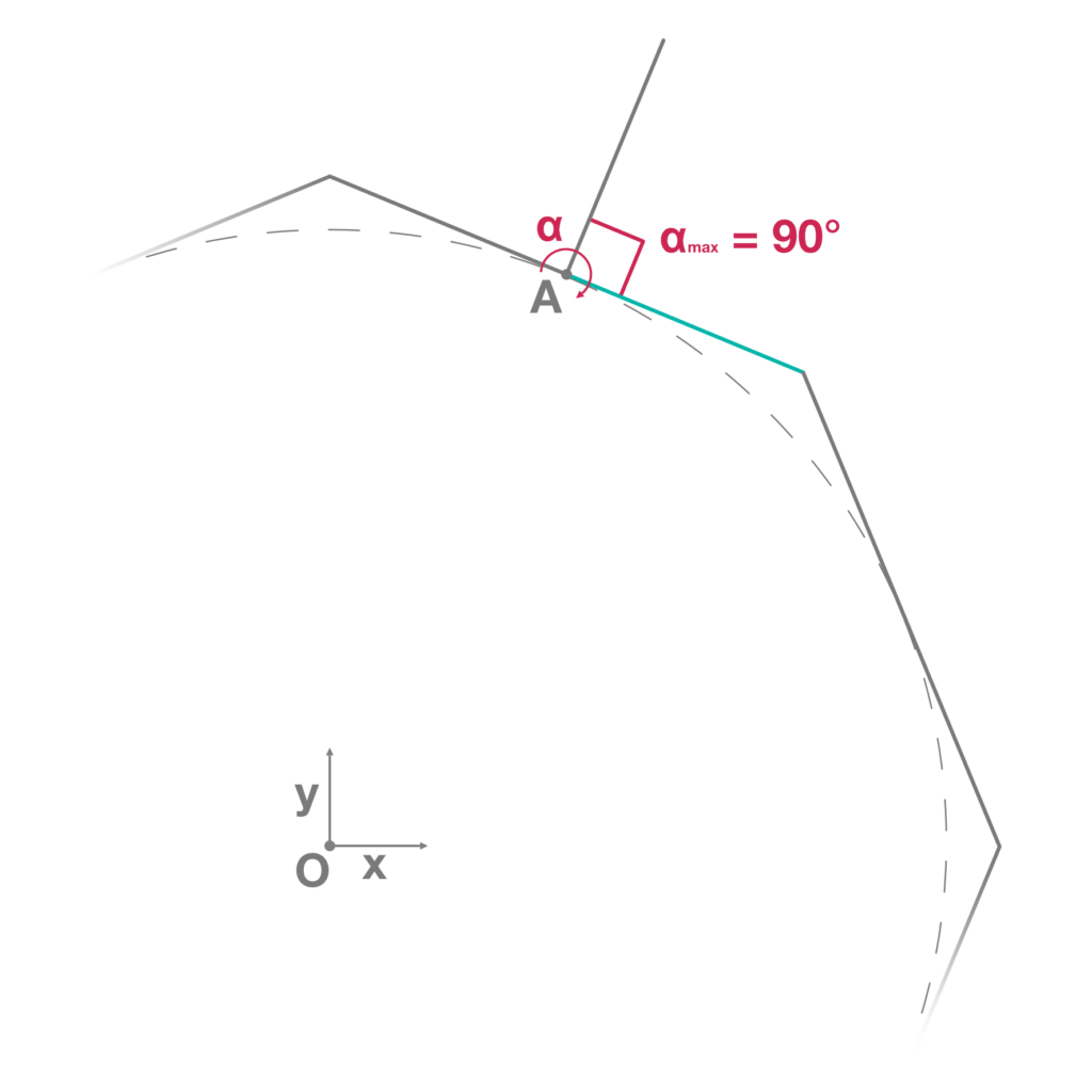
- Rotation of the previous line around the point A by an angular variable α having a domain set from 10° to 90°. This variable is the only one changeable dynamic parameter inside the VR experience, while all the other variables are set in Grasshopper and fixed in Unity. α determines all the available configurations of the geometry. Notice that the starting angle of the domain depends on the physics features of the objects in order to prevent overlapping of material (Fig.3).
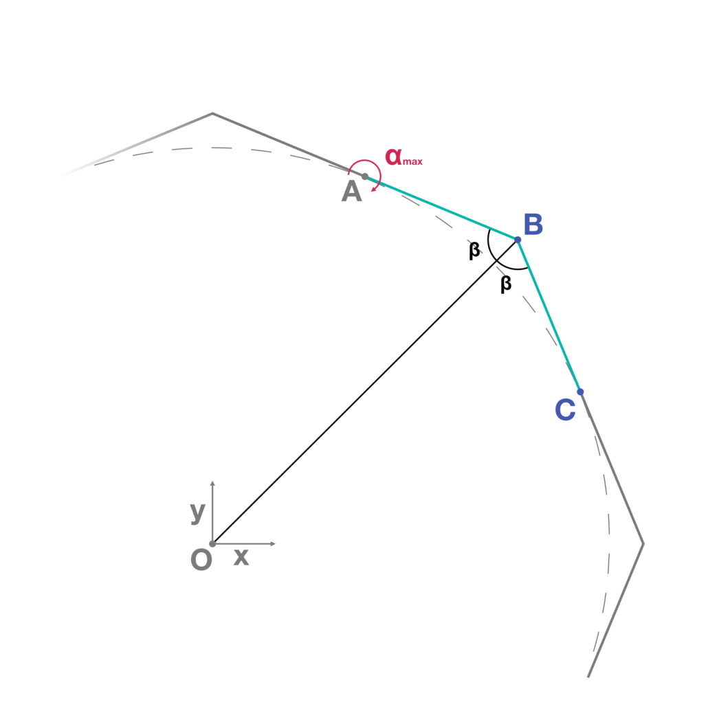
- Detection of the movable endpoint B of the previous line. The same line is then mirrored by a vertical plane passing through the origin of the base polygon and the point B, identifying the point C. Notice that the triangles OAB and OBC are congruent (Fig.4).
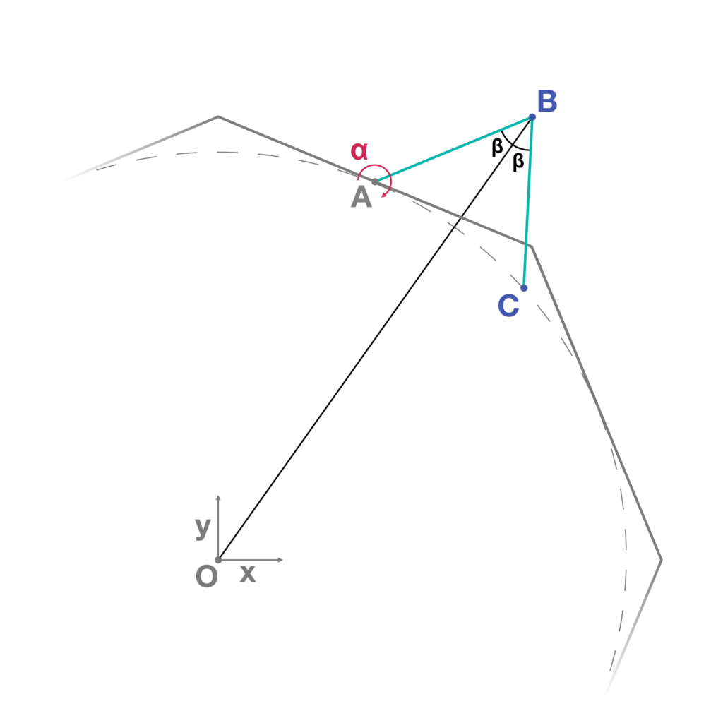
- Varying the parameter α, the point C moves along the reference circle, always getting the congruence between the triangles OAB and OBC and allowing the correct movement of the geometries (Fig.5).
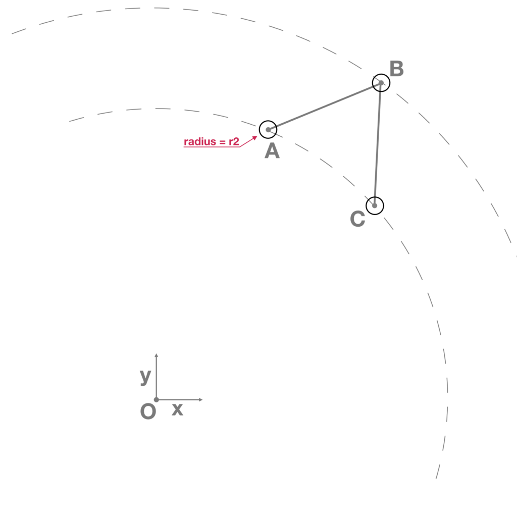
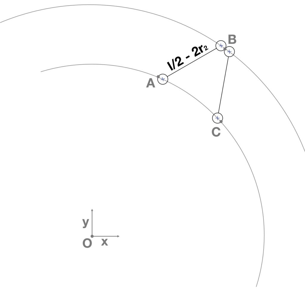
- Construction of three circles from A, B and C. Those circles have a radius equal to the variable r2 which is the radius of the designed cylindrical hinges (Fig.6).
- Intersection between the three previous circles, the reference circle, which has a radius equal to the distance between the origin of the base polygon and the point A, and another circle, which has a variable radius equal to the distance between the origin of the base polygon and the movable point B. These last two circles have the same origin of the base polygon. The intersection generates six points (Fig. 7).
- Construction of four circles from the four selected points. Two lines are then constructed between the couples of center points of the circles. The length of the lines is equal to (l/2) – 2(r2) (Fig.8).
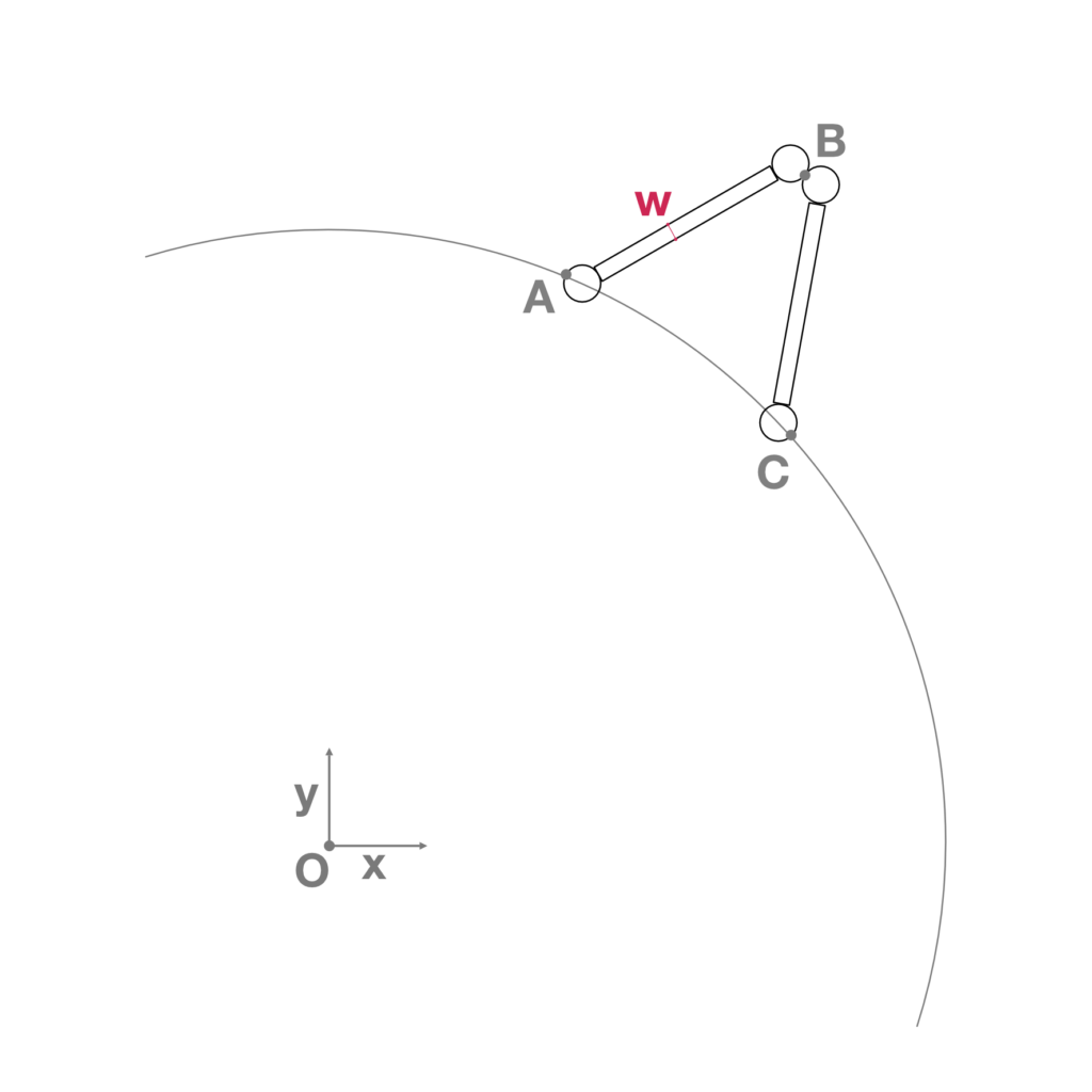
- Construction of two rectangles, from the midpoints of the previous lines, having a length equal to (l/2) – 2(r2) and a width equal to the variable w. The rectangles represent the bases of the panels that compose the final geometry (Fig.9).
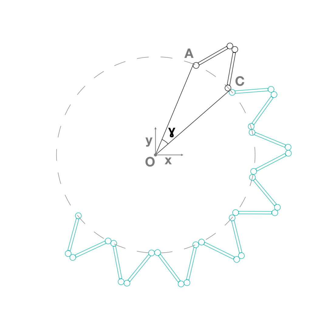
- Polar array of the rectangles and circles by a sweep angle equal to ɣ which depends by the number of the segments of the base polygon (Fig.10).
- Translation of the arrays along the z axis by the variable h which defines the height of the panels and cylinders. The translation vector is defined by the components (0, 0, h) (Fig.11).
- Mesh generation through each couple of rectangles (Fig.12) and through each couple of circles (Fig.13). This operation generates the definitive panels and their cylindrical hinges.
- As it happens for the first geometry of the Piattaforma Zero, the generation of the meshes is made with the C# script downloaded from the ShapeDiver website. Notice that this operation generates directly meshes through the rectangles and circles, avoiding N.U.R.B.S. surfaces that would need to be converted to make them readable in Unity. The base circles of the cylinders are converted in polygons to make the algorithm faster. The final meshes of the cylinders are welded to avoid the jagged effect of the cylinders. Panels and cylinders are then refined using the Combine&Clean component of the plugin Kangaroo Physics, which removes unused and duplicate vertices of the meshes.
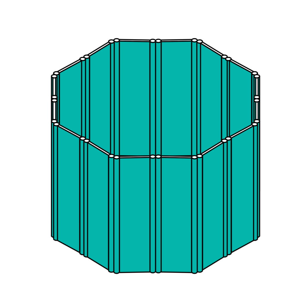
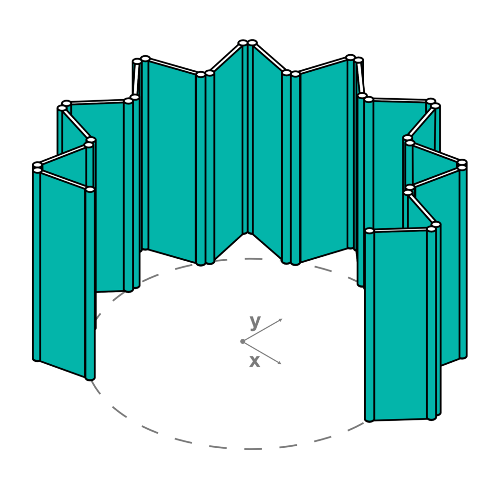
- When the control parameter α assumes the value of 10°, the geometry has its maximum constraint (Fig.14); when it assumes the value of 90°, the geometry is completely deployed and closed (Fig.15); the other values between 10° and 90° lead to the whole set of intermediate configurations of the geometry (Fig.16).
The folding wall is done. Now take your time to play with it so you can make yourself comfortable with this kind of modeling and interactive approach. You can download the commented .gh file from the link below.
Generative Flowchart
Below you can see the recap flowchart pertaining to the generation of the geometry. This can be a useful tool to make the script of the Grasshopper definition easier and to understand the logic behind the generative procedure of this geometric example.
Pio Lorenzo Cocco, November 17, 2020